Introduction to Apache Sedona for R

Introduction

apache.sedona is a sparklyr-based R interface for Apache Sedona. It presents what Apache Sedona has to offer through idiomatic frameworks and constructs in R (e.g., one can build spatial Spark SQL queries using Sedona UDFs in conjunction with a wide range of dplyr expressions), hence making Apache Sedona highly friendly for R users.

Generally speaking, when working with Apache Sedona, one choose between the following two modes:

Manipulating Sedona Spatial Resilient Distributed Datasets with spatial-RDD-related routines
Querying geometric columns within Spatial DataFrames with Sedona spatial UDFs

While the former option enables more fine-grained control over low-level implementation details (e.g., which index to build for spatial queries, which data structure to use for spatial partitioning, etc), the latter is simpler and leads to a straightforward integration with dplyr, sparklyr, and other sparklyr extensions (e.g., one can build ML feature extractors with Sedona UDFs and connect them with ML pipelines using ml_*() family of functions in sparklyr, hence creating ML workflows capable of understanding spatial data).

Because data from spatial RDDs can be imported into Spark DataFrames as geometry columns and vice versa, one can switch between the abovementioned two modes fairly easily.

At the moment apache.sedona consists of the following components:

R interface for Spatial-RDD-related functionalities
- Reading/writing spatial data in WKT, WKB, and GeoJSON formats
- Shapefile reader
- Spatial partition, index, join, KNN query, and range query operations
- Visualization routines
dplyr-integration for Sedona spatial UDTs and UDFs
- See SQL APIs for the list of available UDFs
Functions importing data from spatial RDDs to Spark DataFrames and vice versa

Connect to Spark

To ensure Sedona serialization routines, UDTs, and UDFs are properly registered when creating a Spark session, one simply needs to attach apache.sedona before instantiating a Spark connection. apache.sedona will take care of the rest. For example,

library(sparklyr)
library(apache.sedona)

spark_home <- "/usr/lib/spark"  # NOTE: replace this with your $SPARK_HOME directory
sc <- spark_connect(master = "yarn", spark_home = spark_home)

will create a Sedona-capable Spark connection in YARN client mode, and

library(sparklyr)
library(apache.sedona)

sc <- spark_connect(master = "local")

will create a Sedona-capable Spark connection to an Apache Spark instance running locally.

In sparklyr, one can easily inspect the Spark connection object to sanity-check it has been properly initialized with all Sedona-related dependencies, e.g.,

print(sc$extensions$packages)
#> [1] "org.datasyslab:geotools-wrapper:1.4.0-28.2"
#> [2] "edu.ucar:cdm-core:5.4.2"

and

spark_session(sc) %>%
  invoke("%>%", list("conf"), list("get", "spark.kryo.registrator")) %>%
  print()
#> [1] "org.apache.sedona.viz.core.Serde.SedonaVizKryoRegistrator"

For more information about connecting to Spark with sparklyr, see https://therinspark.com/connections.html and ?sparklyr::spark_connect. Also see Initiate Spark Context and Initiate Spark Session for minimum and recommended dependencies for Apache Sedona.

dplyr workflows

apache.sedona extends sparklyr integrates with dplyr workflows. See the sparklyr cheatsheet

library(dplyr)

Loading data

Copying from R

Data loaded in R can be copied to Spark using copy_to. Columns containing spatial information can be converted to the geometry type in Spark DataFrames (GeometryUDT) with Spark SQL functions such as ST_GeomFromText or ST_GeomFromText, see Vector constructors and Raster input and output.

data <- readr::read_tsv("../../binder/data/county_small.tsv", col_names = FALSE, show_col_types = FALSE)
data %>% glimpse()
#> Rows: 100
#> Columns: 18
#> $ X1  <chr> "POLYGON ((-97.019516 42.004097,-97.019519 42.004933,-97.019527 42…
#> $ X2  <chr> "31", "53", "35", "31", "31", "72", "46", "48", "06", "21", "39", …
#> $ X3  <chr> "039", "069", "011", "109", "129", "085", "099", "327", "091", "05…
#> $ X4  <chr> "00835841", "01513275", "00933054", "00835876", "00835886", "01804…
#> $ X5  <chr> "31039", "53069", "35011", "31109", "31129", "72085", "46099", "48…
#> $ X6  <chr> "Cuming", "Wahkiakum", "De Baca", "Lancaster", "Nuckolls", "Las Pi…
#> $ X7  <chr> "Cuming County", "Wahkiakum County", "De Baca County", "Lancaster …
#> $ X8  <chr> "06", "06", "06", "06", "06", "13", "06", "06", "06", "06", "06", …
#> $ X9  <chr> "H1", "H1", "H1", "H1", "H1", "H1", "H1", "H1", "H1", "H1", "H1", …
#> $ X10 <chr> "G4020", "G4020", "G4020", "G4020", "G4020", "G4020", "G4020", "G4…
#> $ X11 <dbl> NA, NA, NA, 339, NA, 490, NA, NA, NA, NA, 248, NA, NA, 108, 338, N…
#> $ X12 <dbl> NA, NA, NA, 30700, NA, 41980, 43620, NA, NA, NA, 22300, 38380, NA,…
#> $ X13 <dbl> NA, NA, NA, NA, NA, NA, NA, NA, NA, NA, NA, NA, NA, NA, NA, NA, NA…
#> $ X14 <chr> "A", "A", "A", "A", "A", "A", "A", "A", "A", "A", "A", "A", "A", "…
#> $ X15 <dbl> 1477895811, 682138871, 6015539696, 2169240202, 1489645187, 8774836…
#> $ X16 <dbl> 10447360, 61658258, 29159492, 22877180, 1718484, 32509, 17349847, …
#> $ X17 <dbl> 41.91587, 46.29464, 34.35927, 40.78355, 40.17649, 18.18715, 43.667…
#> $ X18 <dbl> -96.78852, -123.42446, -104.36870, -96.68866, -98.04684, -65.87119…

data_tbl <- copy_to(sc, data)

data_tbl
#> # Source: spark<data> [?? x 18]
#>    X1    X2    X3    X4    X5    X6    X7    X8    X9    X10     X11   X12   X13
#>    <chr> <chr> <chr> <chr> <chr> <chr> <chr> <chr> <chr> <chr> <dbl> <dbl> <dbl>
#>  1 POLY… 31    039   0083… 31039 Cumi… Cumi… 06    H1    G4020    NA    NA    NA
#>  2 POLY… 53    069   0151… 53069 Wahk… Wahk… 06    H1    G4020    NA    NA    NA
#>  3 POLY… 35    011   0093… 35011 De B… De B… 06    H1    G4020    NA    NA    NA
#>  4 POLY… 31    109   0083… 31109 Lanc… Lanc… 06    H1    G4020   339 30700    NA
#>  5 POLY… 31    129   0083… 31129 Nuck… Nuck… 06    H1    G4020    NA    NA    NA
#>  6 POLY… 72    085   0180… 72085 Las … Las … 13    H1    G4020   490 41980    NA
#>  7 POLY… 46    099   0126… 46099 Minn… Minn… 06    H1    G4020    NA 43620    NA
#>  8 POLY… 48    327   0138… 48327 Mena… Mena… 06    H1    G4020    NA    NA    NA
#>  9 POLY… 06    091   0027… 06091 Sier… Sier… 06    H1    G4020    NA    NA    NA
#> 10 POLY… 21    053   0051… 21053 Clin… Clin… 06    H1    G4020    NA    NA    NA
#> # … with more rows, and 5 more variables: X14 <chr>, X15 <dbl>, X16 <dbl>,
#> #   X17 <dbl>, X18 <dbl>

data_tbl %>% 
  transmute(geometry = st_geomfromtext(X1)) %>% 
  sdf_schema()
#> $geometry
#> $geometry$name
#> [1] "geometry"
#> 
#> $geometry$type
#> [1] "GeometryUDT"

No automatic translation of sf objects is provided, they need to be converted to text (or binary) format before copying to spark.

data <- sf::st_read("../../binder/data/testPolygon.json")
#> Reading layer `testPolygon' from data source 
#>   `/Users/gregoireleleu/WORK/MISC_CODE/sedona/binder/data/testPolygon.json' 
#>   using driver `GeoJSON'
#> Simple feature collection with 1 feature and 10 fields
#> Geometry type: POLYGON
#> Dimension:     XY
#> Bounding box:  xmin: -87.62176 ymin: 34.83143 xmax: -87.60367 ymax: 34.87344
#> Geodetic CRS:  WGS 84

data %>% glimpse()
#> Rows: 1
#> Columns: 11
#> $ STATEFP  <chr> "01"
#> $ COUNTYFP <chr> "077"
#> $ TRACTCE  <chr> "011501"
#> $ BLKGRPCE <chr> "5"
#> $ AFFGEOID <chr> "1500000US010770115015"
#> $ GEOID    <chr> "010770115015"
#> $ NAME     <chr> "5"
#> $ LSAD     <chr> "BG"
#> $ ALAND    <int> 6844991
#> $ AWATER   <int> 32636
#> $ geometry <POLYGON [°]> POLYGON ((-87.62176 34.8734...

data_tbl <- 
  copy_to(
    sc, 
    data %>% 
    mutate(geometry_wkb = geometry %>% sf::st_as_text()) %>% 
    sf::st_drop_geometry(),
  name = "data",
  overwrite = TRUE
)

data_tbl %>% 
  transmute(geometry = st_geomfromtext(geometry_wkb)) %>% 
  sdf_schema()
#> $geometry
#> $geometry$name
#> [1] "geometry"
#> 
#> $geometry$type
#> [1] "GeometryUDT"

Loading directly in Spark

Loading data in R and then copying it to Spark will most likely not be the optimal method to prepare data for analysis; loading data directly into Spark will often be best.spark_read_* functions are made for this purpose (and extend spark_read_* functions in sparklyr).

data_tbl <- spark_read_geojson(sc, path = "../../binder/data/testPolygon.json", name = "data")

data_tbl %>% 
  glimpse()
#> Rows: ??
#> Columns: 11
#> Database: spark_connection
#> $ geometry <list> <<environment: 0x1288c4cf8>>, <<environment: 0x12886ecf8>>, …
#> $ STATEFP  <chr> "01", "01", "01", "01", "01", "01", "01", "01", "01", "01", "…
#> $ COUNTYFP <chr> "077", "045", "055", "089", "069", "073", "101", "015", "069"…
#> $ TRACTCE  <chr> "011501", "021102", "001300", "001700", "041400", "010801", "…
#> $ BLKGRPCE <chr> "5", "4", "3", "2", "1", "4", "3", "1", "2", "3", "2", "4", "…
#> $ AFFGEOID <chr> "1500000US010770115015", "1500000US010450211024", "1500000US0…
#> $ GEOID    <chr> "010770115015", "010450211024", "010550013003", "010890017002…
#> $ NAME     <chr> "5", "4", "3", "2", "1", "4", "3", "1", "2", "3", "2", "4", "…
#> $ LSAD     <chr> "BG", "BG", "BG", "BG", "BG", "BG", "BG", "BG", "BG", "BG", "…
#> $ ALAND    <chr> "6844991", "11360854", "1378742", "1040641", "8243574", "1303…
#> $ AWATER   <chr> "32636", "0", "247387", "0", "0", "9989", "0", "0", "159228",…

data_tbl %>% 
  select(geometry) %>% 
  sdf_schema()
#> $geometry
#> $geometry$name
#> [1] "geometry"
#> 
#> $geometry$type
#> [1] "GeometryUDT"

Manipulating

The dbplyr interface transparently translates dbplyr worklfows into SQL, and gives access to all Apache Sedona SQL functions:

Results are then collected back into R with collect.

## ! ST_FlipCoordinates needs to be called before st_transform as by default, this function uses lat/lon order
data_tbl %>% 
  mutate(
    ALAND = ALAND %>% as.numeric(),
    AWATER = AWATER %>% as.numeric(),
    area = ALAND + AWATER,
    geometry_proj = st_transform(ST_FlipCoordinates(geometry), "epsg:4326", "epsg:5070", TRUE),
    area_geom = st_area(geometry_proj)
    ) %>% 
  select(STATEFP, COUNTYFP, area, area_geom) %>% 
  head() %>% 
  collect()
#> # A tibble: 6 × 4
#>   STATEFP COUNTYFP     area area_geom
#>   <chr>   <chr>       <dbl>     <dbl>
#> 1 01      077       6877627  6885810.
#> 2 01      045      11360854 11372509.
#> 3 01      055       1626129  1615070.
#> 4 01      089       1040641  1072135.
#> 5 01      069       8243574  8250531.
#> 6 01      073       1313587  1302813.

Geometries need to be converted to a serializable (text or binary) format before collect is called:

## Setting the CRS in R post-collect
data_tbl %>% 
  mutate(
    area = st_area(st_transform(ST_FlipCoordinates(geometry), "epsg:4326", "epsg:5070", TRUE)),
    geometry_wkb = geometry %>% st_asBinary()
    ) %>% 
  select(COUNTYFP, geometry_wkb) %>% 
  head() %>% 
  collect() %>% 
  sf::st_as_sf(crs = 4326)
#> Simple feature collection with 6 features and 1 field
#> Geometry type: POLYGON
#> Dimension:     XY
#> Bounding box:  xmin: -87.62176 ymin: 31.22179 xmax: -85.33003 ymax: 34.87344
#> Geodetic CRS:  WGS 84
#> # A tibble: 6 × 2
#>   COUNTYFP                                                          geometry_wkb
#> * <chr>                                                            <POLYGON [°]>
#> 1 077      ((-87.62176 34.87344, -87.61754 34.87337, -87.6123 34.87334, -87.604…
#> 2 045      ((-85.71902 31.2979, -85.71563 31.3052, -85.71427 31.3071, -85.69999…
#> 3 055      ((-86.00069 34.00537, -85.99884 34.00977, -85.99801 34.0104, -85.987…
#> 4 089      ((-86.57417 34.72738, -86.56268 34.72713, -86.5628 34.72387, -86.562…
#> 5 069      ((-85.38287 31.23477, -85.37651 31.2347, -85.37143 31.23569, -85.365…
#> 6 073      ((-86.77326 33.49818, -86.77416 33.49972, -86.77005 33.50257, -86.77…

## Setting the CRS in Spark (and using EWKT to keep it)
data_tbl %>% 
  mutate(
    area = st_area(st_transform(ST_FlipCoordinates(geometry), "epsg:4326", "epsg:5070", TRUE)),
    geometry_ewkt = geometry %>% st_setsrid(4326) %>% st_asewkt()
    ) %>% 
  select(COUNTYFP, geometry_ewkt) %>% 
  head() %>% 
  collect() %>% 
  sf::st_as_sf(wkt = "geometry_ewkt") 
#> Simple feature collection with 6 features and 1 field
#> Geometry type: POLYGON
#> Dimension:     XY
#> Bounding box:  xmin: -87.62176 ymin: 31.22179 xmax: -85.33003 ymax: 34.87344
#> Geodetic CRS:  WGS 84
#> # A tibble: 6 × 2
#>   COUNTYFP                                                         geometry_ewkt
#>   <chr>                                                            <POLYGON [°]>
#> 1 077      ((-87.62176 34.87344, -87.61754 34.87337, -87.6123 34.87334, -87.604…
#> 2 045      ((-85.71902 31.2979, -85.71563 31.3052, -85.71427 31.3071, -85.69999…
#> 3 055      ((-86.00069 34.00537, -85.99884 34.00977, -85.99801 34.0104, -85.987…
#> 4 089      ((-86.57417 34.72738, -86.56268 34.72713, -86.5628 34.72387, -86.562…
#> 5 069      ((-85.38287 31.23477, -85.37651 31.2347, -85.37143 31.23569, -85.365…
#> 6 073      ((-86.77326 33.49818, -86.77416 33.49972, -86.77005 33.50257, -86.77…

Writing

Collected results can be saved from R. In many cases it will be more efficient to write results directly from Spark. The spark_write_* (see docs) functions are made for this purpose (and extend spark_write_* functions in sparklyr).

dest_file <- tempfile() ## Destination folder
data_tbl %>% 
  filter(str_sub(COUNTYFP, 1, 2) == "00") %>% 
  spark_write_geoparquet(path = dest_file)

dest_file %>% dir(recursive = TRUE)
#> [1] "_SUCCESS"                                                           
#> [2] "part-00000-589c9d07-373c-4f56-8e1d-c68eb9be4782-c000.snappy.parquet"

The output can be partitioned by the columns present in the data:

dest_file <- tempfile()  ## Destination folder
data_tbl %>% 
  filter(str_sub(COUNTYFP, 1, 2) == "00") %>% 
  spark_write_geoparquet(path = dest_file, partition_by = "COUNTYFP")

dest_file %>% dir(recursive = TRUE)
#> [1] "_SUCCESS"                                                                        
#> [2] "COUNTYFP=001/part-00000-fe1d05d3-8a10-4f5c-8be6-807e221902c5.c000.snappy.parquet"
#> [3] "COUNTYFP=003/part-00000-fe1d05d3-8a10-4f5c-8be6-807e221902c5.c000.snappy.parquet"
#> [4] "COUNTYFP=005/part-00000-fe1d05d3-8a10-4f5c-8be6-807e221902c5.c000.snappy.parquet"
#> [5] "COUNTYFP=007/part-00000-fe1d05d3-8a10-4f5c-8be6-807e221902c5.c000.snappy.parquet"
#> [6] "COUNTYFP=009/part-00000-fe1d05d3-8a10-4f5c-8be6-807e221902c5.c000.snappy.parquet"

Spark DataFrames

Spark DataFrames provide a higher level API than RDDs, and can be used with SQL queries. sparklyr and apache.sedona automatically wrap Spark DataFrames in dplyr tbls to work in dplyr workflows.

data_tbl %>% class()
#> [1] "tbl_spark" "tbl_sql"   "tbl_lazy"  "tbl"

You can get to the underlying Spark DataFrame (SDF) with sparklyr::spark_dataframe, to be used for example in with spakrlyr::invoke to call SDF methods within Spark.

sdf <- data_tbl %>% spark_dataframe()
sdf
#> <jobj[162]>
#>   org.apache.spark.sql.Dataset
#>   [geometry: geometry, STATEFP: string ... 9 more fields]

RDD workflows

What are `SpatialRDD`s?

SpatialRDDs are basic building blocks of distributed spatial data in Apache Sedona. A SpatialRDD can be partitioned and indexed using well-known spatial data structures to facilitate range queries, KNN queries, and other low-level operations. One can also export records from SpatialRDDs into regular Spark DataFrames, making them accessible through Spark SQL and through the dplyr interface of sparklyr.

Creating a SpatialRDD

NOTE: this section is largely based on Spatial RDD Scala tutorial, except for examples have been written in R instead of Scala to reflect usages of apache.sedona.

Currently SpatialRDDs can be created in apache.sedona by reading a file in a supported geospatial format (sedona_read_* functions), or by extracting data from a Spark SQL query.

For example, the following code will import data from arealm-small.csv into a SpatialRDD:

pt_rdd <- sedona_read_dsv_to_typed_rdd(
  sc,
  location = "../../binder/data/arealm-small.csv",
  delimiter = ",",
  type = "point",
  first_spatial_col_index = 1,
  has_non_spatial_attrs = TRUE
)

Records from the example arealm-small.csv file look like the following:

testattribute0,-88.331492,32.324142,testattribute1,testattribute2
testattribute0,-88.175933,32.360763,testattribute1,testattribute2
testattribute0,-88.388954,32.357073,testattribute1,testattribute2

As one can see from the above, each record is comma-separated and consists of a 2-dimensional coordinate starting at the 2nd column and ending at the 3rd column. All other columns contain non-spatial attributes. Because column indexes are 0-based, we need to specify first_spatial_col_index = 1 in the example above to ensure each record is parsed correctly.

In addition to formats such as CSV and TSV, currently apache.sedona also supports reading files in WKT (Well-Known Text), WKB (Well-Known Binary), Shapefile and GeoJSON formats. See sedona_read_wkt() for details.

Conversion to and from SpatialRDD

One can also run to_spatial_rdd() to extract a SpatialRDD from a Spark SQL query, e.g. the query below will extract a spatial column named "geom" from the Sedona spatial SQL query above and store it in a SpatialRDD object.

library(dplyr)

sdf <- tbl(
  sc,
  sql("SELECT ST_GeomFromText('POINT(-71.064544 42.28787)') AS `geom`, \"point\" AS `type`")
)

spatial_rdd <- sdf %>% to_spatial_rdd(spatial_col = "geom")
spatial_rdd
#> $.jobj
#> <jobj[170]>
#>   org.apache.sedona.core.spatialRDD.SpatialRDD
#>   org.apache.sedona.core.spatialRDD.SpatialRDD@21e80d8a
#> 
#> $.state
#> <environment: 0x12fd21bc0>
#> 
#> attr(,"class")
#> [1] "spatial_rdd"

A SpatialRDD can be converted into a Spark DataFrame with sdf_register (generic method from sparklyr).

spatial_sdf <- spatial_rdd %>% sdf_register(name = "my_table")
spatial_sdf
#> # Source: spark<my_table> [?? x 2]
#>   geometry                      type 
#>   <list>                        <chr>
#> 1 <POINT (-71.064544 42.28787)> point

Visualization

An important part of apache.sedona is its collection of R interfaces to Sedona visualization routines. For example, the following is essentially the R equivalent of this example in Scala.

resolution_x <- 1000
resolution_y <- 600
boundary <- c(-126.790180, -64.630926, 24.863836, 50.000)

pt_rdd <- sedona_read_dsv_to_typed_rdd(
  sc,
  location = "../../core/src/test/resources/arealm.csv",
  type = "point"
)
polygon_rdd <- sedona_read_dsv_to_typed_rdd(
  sc,
  location = "../../core/src/test/resources/primaryroads-polygon.csv",
  type = "polygon"
)
pair_rdd <- sedona_spatial_join_count_by_key(
  pt_rdd,
  polygon_rdd,
  join_type = "intersect"
)

overlay <- sedona_render_scatter_plot(
  polygon_rdd,
  resolution_x,
  resolution_y,
  output_location = tempfile("scatter-plot-"),
  boundary = boundary,
  base_color = c(255, 0, 0),
  browse = FALSE
)

sedona_render_choropleth_map(
  pair_rdd,
  resolution_x,
  resolution_y,
  output_location = "./choropleth-map",
  boundary = boundary,
  overlay = overlay,
  # vary the green color channel according to relative magnitudes of data points so
  # that the resulting map will show light blue, light purple, and light gray pixels
  color_of_variation = "green",
  base_color = c(225, 225, 255)
)

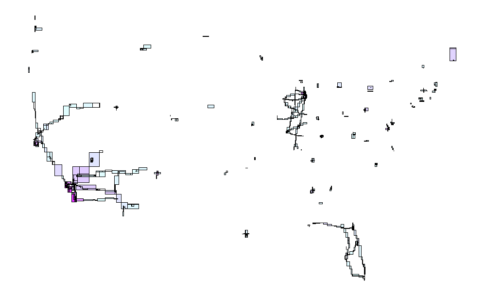
It will create a scatter plot, and then overlay it on top of a choropleth map, as shown below:

See ?apache.sedona::sedona_render_scatter_plot, ?apache.sedona::sedona_render_heatmap, and ?apache.sedona::sedona_render_choropleth_map for more details on visualization-related R interfaces currently implemented by apache.sedona.

Advanced parameters

Various advanced parameters can be set in Apache Sedona, see parameters

Through the sparklyr config:

config <- spark_config()
config[["sedona.global.index"]] <- FALSE

sc <- spark_connect(master = "local", config = config)
#> ℹ Using Sedona jars listed in SEDONA_JAR_FILES variable (see Sys.getenv("SEDONA_JAR_FILES"))

Check

invoke_new(sc, "org.apache.sedona.core.utils.SedonaConf", invoke(spark_session(sc), "conf")) 
#> <jobj[53]>
#>   org.apache.sedona.core.utils.SedonaConf
#>   Sedona Configuration:
#> useIndex: true
#> indexType: QUADTREE
#> joinSparitionDominantSide: LEFT
#> joinBuildSide: LEFT
#> joinApproximateTotalCount: -1
#> datasetBoundary: Env[0.0 : 0.0, 0.0 : 0.0]
#> fallbackPartitionNum: -1
#> joinGridType: KDBTREE
#> autoBroadcastJoinThreshold: 10485760

Or change at runtime:

spark_session(sc) %>% 
  invoke("conf") %>% 
  invoke("set", "sedona.global.index","true")
#> NULL

invoke_new(sc, "org.apache.sedona.core.utils.SedonaConf", invoke(spark_session(sc), "conf")) 
#> <jobj[57]>
#>   org.apache.sedona.core.utils.SedonaConf
#>   Sedona Configuration:
#> useIndex: true
#> indexType: QUADTREE
#> joinSparitionDominantSide: LEFT
#> joinBuildSide: LEFT
#> joinApproximateTotalCount: -1
#> datasetBoundary: Env[0.0 : 0.0, 0.0 : 0.0]
#> fallbackPartitionNum: -1
#> joinGridType: KDBTREE
#> autoBroadcastJoinThreshold: 10485760